OptiNod Academy
Wyckoff Method — Applying It in the Crypto and Algorithmic Era (Part 5)
How classic Wyckoff features change in a market that adds 24-hour trading, the funding rate, on-chain data, and liquidity pools.
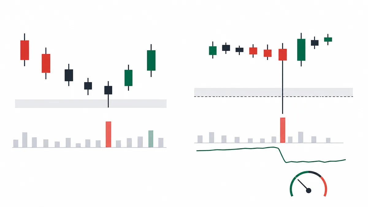
The Composite Operator (the large-player hypothesis) is unchanged. It only changed from a person to an algorithm. What differs is the way the traces are left.
The first four parts covered the core of Wyckoff (a single pressure called the Composite Operator), the four-stage cycle, the nine events and the stage structure, and volume spread analysis and Weis Wave. This article covers how those tools change in today's 24-hour crypto market and in a market dominated by algorithmic trading. The conclusion is simple. The essence works the same way. What changes together is the shape in which the traces appear, and the time unit.
Popular readings split two ways. One side concludes that "Wyckoff is a tool from the 1930s New York Stock Exchange floor, so it does not fit a BTC market that never sleeps." The other asserts that "it works well applied exactly as in the classic form." Each sees only one side. The mechanism works the same way, but the features show up in a clearly different shape. If a 1930s selling climax was an event built across one or two daily bars, BTC's selling climax on August 5, 2024 finished inside a single day, in two or three 4-hour bars.
This article returns to four points.
- Session boundaries disappear: 24-hour trading erases session boundaries, and Phase B stretches out to weekly and monthly units.
- New Wyckoff indicators: The funding rate and open interest (OI) work as new Wyckoff indicators that supplement classic volume.
- Trigger coordinates move: The trigger coordinates of a Spring and of the upthrust after distribution move from the price line to the location of a liquidity pool.
- On-chain context: On-chain whale-wallet tracking shows, in the data, the movement of an actor that can be read as the Composite Operator.

In a 24-Hour Market, Stage B Stretches Out to the Weekly Chart
In classic Wyckoff, accumulation stage B in an NYSE stock usually forms over three to twelve weeks. The market is open only 6.5 hours a day and is closed on weekends and holidays, so the process of large players gathering inventory naturally finishes inside a quarter. Calendar events such as earnings, dividends, and option expiration also act as outside reference points for when a stage will end.
Crypto is different. BTC trades 24 hours a day, 365 days a year, and has no session boundary. That one difference greatly lengthens the period over which stage B unfolds. The seven months BTC spent ranging between $24,000 and $32,000 from mid-March to mid-October 2023 is an abnormally long stage B by classic standards, but in crypto it is standard. On the daily chart over that same period the range can look as if it never formed, but widen to the weekly chart and a clear accumulation pattern shows up.
The practical conclusion to draw from this change of time unit is to raise the analysis timeframe by one step. The cycle that was watched on the daily chart in the 1930s has to be watched on the weekly chart in crypto, and the daily chart drops to a lower timeframe and is used only for the entry trigger. After the August 5, 2024 low of $2,111, ETH entered a range in the $2,100-$2,800 area and broke $3,000 on November 9 of that year. On the weekly chart, the sequence runs from the spring to a sign of strength to the retest confirmation. On the daily chart alone, the whole three months is a grind of whipsaws inside the range.
The second result of lost session boundaries is the weekend liquidity trap. On Saturday and Sunday, institutional desks are closed and volume falls to around 50% of weekday levels, and range breaks happen often then. Volume is thin, so a small order pushes price out of the range, and the pattern of a return back inside the range during Monday's Asian session repeats. Treat that false break as a spring and enter, and you land squarely in the whipsaw.
Flash Crash — The Compressed Form of a Selling Climax
A classic selling climax is built across one or two daily bars. The Dow on October 28 and 29, 1929, and the SPX on October 19, 1987, were both crash events on a daily scale. In a 24-hour market, that selling climax compresses into a span of hours, and the compressed selling climax is the flash crash.
On August 5, 2024, BTC fell 16% in eight hours, from $58,300 to $49,000. It was a forced liquidation cascade set off by the unwind of the Japan carry trade, and volume on three 4-hour bars expanded sharply to 4-6 times the prior 20-bar average. Every feature of a classic selling climax — sharply higher volume, wide bars, a close near the top of the bar (a trace that buyers had come in) — showed up the same way on the 4-hour chart. After that, the automatic rally ran quickly to $56,000, and on August 7 a secondary test printed near $54,600 with volume down.
The key to an entry after a selling climax that arrived as a flash crash is to check the strength of the automatic rally. If price does not recover 8% or more from the selling-climax low within 24-48 hours, treat it as the first stage of further selling. BTC's first sharp drop near $21,900 on June 13, 2022 came on sharply higher volume and looked like a selling climax, but the rebound over the next 48 hours was only 6.6%, so the automatic rally was weak, and the drop continued to $17,600 on June 18. That $17,600 print was the real selling climax.
The second trap of a compressed selling climax is the fake selling climax made by a liquidation cascade. Forced liquidations in the perp market call more liquidations, a domino that drops price 10-15% in four hours, and it happens once or twice a quarter. That cascade is closer to leverage coming unwound all at once, and the source of the extra volume is concentrated on the forced-selling side.
To separate a real selling climax from a liquidation cascade, look at spot volume and perp volume separately. Spot volume has to expand sharply as well before it can be read as the selling climax of a real accumulation. If only the perp expands and spot stays at its usual level, it is just a leverage-liquidation phase.
Funding Rate and Open Interest — The New Wyckoff Volume
In classic Wyckoff, volume was the primary information for reading who was acting and what they intended. One volume bar was the tool for judging whether large players had come in or left. In the crypto perp market, that information splits into two streams: the funding rate and open interest.
The funding rate is the rate that long and short positions pay each other to keep the perpetual future (perp) aligned with spot. It settles every eight hours and usually stays between -0.01% and +0.01%. Where this rate exceeds ±0.05%, it shows in a number which way the market is leaning.
- Positive extreme: Longs pay shorts a large fee. The whole market is overcrowded on the long side, and that is a feature of distribution.
- Negative extreme: A new measure of capitulation.
In the week before BTC made a new high at $73,800 in March 2024, the funding rate on every major exchange was +0.08% to +0.12%, five times or more the one-month average. Price made a new high, but the fact that the capital which made that high was crowded too far to one side showed up directly in the funding rate. A 19% correction then ran through April 17, and funding normalized to +0.005%.
Open interest is the total notional value of perp positions that have not been closed. The absolute value of OI alone is a poor basis for a trade, but the direction of the OI change read together with the direction of price gives the same information as Wyckoff volume.
- Price up + OI up: New capital is coming in and building the trend.
- Price up + OI flat or down: Price is rising only on the closing pressure of existing shorts. The force behind the rise is weak, so once the closing is finished, price soon sits back down.
When ETH stalled near $4,000 in December 2024 and started to correct, OI on December 16, the second attempt at $4,000, was clearly lower than on the first attempt. Price reached the same spot a second time, but the open interest behind that move was smaller than the first. This OI divergence shows the same information as an upthrust-after-distribution feature, one beat earlier.

Liquidity Pools — Where Springs and Upthrusts After Distribution Actually Happen
In classic Wyckoff, a spring is the price move in Phase C that briefly leaves the bottom of the range and comes straight back. It is the place where large players shake out the last sellers and finish the accumulation. In today's market, dominated by algorithmic trading, the trigger coordinate of that spring moves from the price line to a liquidity coordinate.
A liquidity pool is a price area where stop orders are piled up in size. They mostly build in these places.
- Below the range low: Just under a clear support line.
- Below the prior swing low: Just under the previous swing low.
- Below round numbers: Just under round numbers such as $50,000 or $60,000.
Algorithmic trading systems (market makers and the active bots of hedge funds) find these liquidity coordinates directly, and price tends to be pulled toward the price area where liquidity is concentrated. While it is being pulled, stop orders trigger and automatic selling floods in. The algorithm takes that sell supply at a low price, then returns price to the range. That is the mechanism of a spring today.

While SOL held a $210 to $220 range in November 2024, a large cluster of stops had built just below the $210 support. On November 14, price briefly fell toward $207. Stops triggered, automatic selling flooded in, and within the same day price recovered to around $222. That is the standard shape of an algorithm-triggered spring, and over the next several days SOL continued the trend above the range.
The upthrust after distribution works by the same mechanism in the opposite direction. A large cluster of short stops (forced-buy triggers) sits just above the top of the range. When an algorithm pulls price up there and sets off short liquidations, large players use the buy flow from those liquidations for distribution (selling). So where a spring or an upthrust after distribution will show up has to be estimated in advance by seeing where the liquidity has built. Tools such as Coinglass and Hyblock show a heatmap of the liquidity distribution, and the liquidity coordinates piled near the bottom and top of the range are where the next spring or upthrust after distribution comes out.
BTC has been ranging between $90,000 and $100,000 on the daily chart for four weeks or more,and the Coinglass liquidity heatmap shows a large cluster of long stops piled near $89,500.4-hour OI is clearly trending up through the range (new capital coming in),and the funding rate is -0.02% or lower (the market is crowded on the short side).Enter long at the close of the bar that briefly breaks below $89,500 and returns inside the range within four hours.Place the stop with an extra $200 of room below the low of the break bar.If price fails to return inside the range within four hours, or if OI falls further after the break, treat the trend as changed and exit.
On-Chain Whale Movement — A Clue for Reading the Composite Operator
The biggest weakness of classic Wyckoff was that the identity of the Composite Operator could be known only as a guess. On the 1930s NYSE, nobody knew who the large player was, and that presence had to be tracked backward from volume and price action. On-chain data for BTC and ETH turns that guess into data you can observe.
On-chain data publishes every trade at the wallet-address level, and analytics firms (Glassnode, CryptoQuant, Nansen) classify wallets that hold large capital as whale wallets and track deposits and withdrawals in real time. The two flows map exactly onto classic Wyckoff distribution and accumulation.
- Large transfers to exchanges: A signal of intent to sell, corresponding to classic Wyckoff distribution.
- Large withdrawals to cold wallets: A signal of a turn toward long-term holding, corresponding to classic Wyckoff accumulation.
During the days BTC made its selling climax at $17,600 in June 2022, Glassnode's Long-Term Holder Supply rose steeply. The fact that long-term holders' BTC holdings grew while price was crashing was strong evidence that large players were taking the panic selling. In a classic market, the sharp rise in selling-climax volume would have had to be read as a guess. On-chain data shows, wallet by wallet, who took that supply.
The trap of on-chain data is that the assets it can be used on are limited to BTC, ETH, SOL, and some majors. On smaller altcoins, the on-chain activity itself is wash trading or the project team's own trading, so the Wyckoff features are hard to trust. Also, once a BTC ETF exists, the real institutional capital flow is captured in ETF fund flows rather than on-chain. So from January 2024 on, BTC analysis has to read on-chain data together with ETF net inflows and outflows (especially IBIT and FBTC) before the full picture of the large players is visible.

In Algorithmic Markets, the Timeframes Where Wyckoff Works Split Apart
In a market dominated by algorithmic trading, Wyckoff does not work equally well on every timeframe. Strength differs by timeframe.
- Weekly and higher: This is where the essence of Wyckoff shows up most cleanly. Algorithms dominate the fine moves of minutes and hours, but a weekly trend still moves on the actual intent of large capital. Accumulation and distribution patterns seen on the weekly charts of BTC, ETH, and SOL work as classic Wyckoff.
- Daily: This is where algorithmic interference starts in earnest. The shape of the features holds, but the funding rate and OI have to be read together to tell real from fake.
- 4-hour: This is where compressed selling climaxes, springs, and upthrusts after distribution show up often, and they become usable only when liquidity-coordinate analysis is read with them.
Below one hour, Wyckoff analysis does not work. More than 80% of patterns that look like a spring on the 1-hour chart are simply the result of an algorithmic liquidity hunt, and they have nothing to do with a real accumulation stage. Anyone reading Wyckoff on a short timeframe keeps getting caught on the algorithm's bait.
There are also differences by session.
- Asia hours (UTC 0-8): Liquidity is thinnest and algorithmic liquidity hunts happen most often, so range breaks in this window have a clearly higher whipsaw rate.
- Europe-U.S. overlap (UTC 13-17): Institutional desks are all active, so real trend moves happen most often.
So when you check whether a Wyckoff signal is real, it is more stable to wait through this window.
Accumulation stage B, formed on the ETH weekly chart in a range for six months or more, is confirmed,and a stage C spring candidate forms on the daily chart.At the same time the funding rate is -0.04% or lower, a clear negative skew,and Glassnode's Long-Term Holder Supply has increased 1.5% or more over the last 30 days.If 4-hour OI dips once on the spring bar and recovers in the next four hours, absorption of capital is confirmed.Enter long at the close of the spring bar, but start the entry size at half the usual size.Place the stop 1.0 times ATR(14) below the low of the spring bar.If the next weekly bar closes below the spring low, or if funding flips immediately to +0.05% or higher, drop that read and exit.
Starting the entry size at half is the point. A spring in an algorithmic market is harder to sort into real or fake than in the classic market. Scaling in, adding size each time another confirmation arrives, is the safer path. Taking a full position at once leaves you fully exposed to a fake spring. If a sign-of-strength bar is confirmed the following week, add size, and add once more on the final retest-confirmation pullback.
The Composite Operator Is an Analytical Assumption for Reading the Net Force
The Composite Operator is not a claim that one real actor exists. It is an analytical assumption that reads the net force of large capital, as it shows up in price and volume, as if it were one actor. Algorithmic orders can take part in that net force, but that does not mean every participant has turned into one piece of code. As in Part 1, confirm the observable traces in price and volume, and do not settle who is behind them.
The classic nine events still work. Only the shape has changed.
- Selling climax: It has changed into a flash crash.
- Automatic rally: It has changed into the automatic rally after selling is exhausted.
- Spring: It has changed into the result of a liquidity hunt.
- Upthrust after distribution: It has changed into a short-liquidation trigger.
In the same vein, the wide bar-range bar of volume spread analysis has been compressed into a 4-hour form where volume expands sharply, and the cumulative curve of Weis Wave can be supplemented with the funding rate and the OI flow.
The trap you meet most often is forgetting the essence and seeing only the shape of the feature. Losses come from taking an algorithm-made fake spring as real, misreading a liquidation cascade as a selling climax, or reading wash-trading volume as accumulation. Wyckoff works properly in an algorithmic market only when the intent of the Composite Operator is the reference point and price, volume, funding, OI, and on-chain data are cross-checked together. That cross-check is the standard that ties together the tools built in the first five parts. Parts 6 and 7 carry it on into a roadmap and a scanner.
