OptiNod Academy
The Kelly Criterion — Separate Loss Risk From Position Allocation
The binary Kelly fraction measures equity lost on a losing bet. Translate a separately chosen risk limit into position size using the entry-to-stop distance, and assess uncertainty, drawdowns, and joint exposure before sizing.
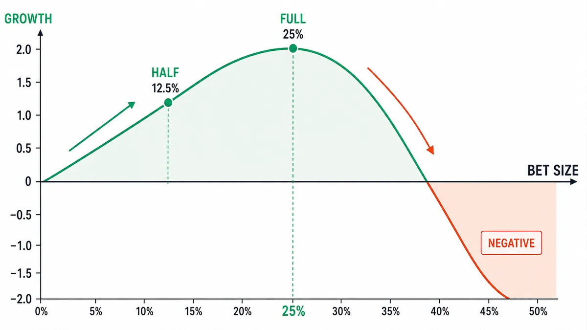
The binary Kelly fraction describes the equity lost on a losing bet. Turning that figure into a trading position requires a separate decision about acceptable loss and the distance from entry to stop.
The Kelly criterion asks how to size repeated bets to maximize long-run compound growth under a specified model. In the simple binary model, each win earns +bR and each loss costs −1R, with win probability p and loss probability q = 1 − p. Its optimal fraction is f* = p − q/b. For the hypothetical values p = 0.55 and b = 1.5, the result is f* = 0.25. Here, 25% is the fraction of equity lost on a losing bet. It is not an instruction to invest 25% of equity in an asset.
That distinction changes the sizing decision. For a linear position, a separately chosen planned loss risk r and an entry-to-stop distance d, both expressed as fractions, give a notional allocation of approximately w = r/d. A 1% planned loss with a stop 2.5% from entry implies 40% of equity in notional exposure before fees, slippage, gaps, and financing costs. The binary Kelly calculation alone does not choose that 1% limit or ensure the stop will contain the loss.
Kelly maximizes expected log wealth within its assumptions. It does not set a maximum acceptable drawdown, and an estimate from past trades is neither a proven optimum for future trading nor a safe ceiling. Before using a Kelly estimate, identify what a loss means, test how uncertain the return distribution is, and set limits for the account and its simultaneous positions.

Kelly Maximizes Expected Log Growth Under Its Model
The Kelly criterion does not maximize the expected profit of one bet. In the binary model, expected profit is positive when pb > q, or p > 1/(1+b). A win rate above 50% is the relevant threshold only at even odds, where b = 1. If the stake is limited to between 0% and 100% and you maximize only expected profit, betting the entire account is the answer under that condition, but one loss wipes the account out. Expected log growth instead accounts for the compounding damage from losses.
The distinction matters because, under compounding, one large loss raises the burden of what comes next. Recovering from a 50% loss requires a 100% gain. For our hypothetical 55% win rate and 1.5 payoff, expected log growth per bet is g(f) = 0.55 ln(1+1.5f) + 0.45 ln(1−f). At full Kelly, f = 0.25, it is 0.0456926; at twice that fraction, f = 0.50, it is −0.0041275. These are expected logarithmic growth values using natural logs, not expected simple percentage returns. Twice Kelly produces slightly negative growth in this example; a zero-growth point at exactly twice Kelly is not a universal rule.
A market selloff helps explain why the loss model matters, but cannot establish a strategy's Kelly fraction. In Binance BTCUSDT spot daily data, using UTC candles, May 19, 2021 opened at 42,849.78 USDT and the intraday low reached 30,000 USDT, about 30% below the open. The April 14 high had been 64,854 USDT. These prices show the scale of the market move; account losses would also depend on exposure, leverage, entries, exits, and fills. The fall does not by itself move a strategy to the right of its Kelly peak. The first check is whether the loss size in the calculation still holds in a move like this.
Full Kelly Can Produce Drawdowns Beyond an Account's Tolerance
Full Kelly is the optimum of expected log growth. It is not a rule that caps maximum drawdown. In the hypothetical model above, staking 25% of current equity and losing three times in a row leaves 0.75³ = 0.421875, about 42.19% of the starting equity. With no other trades in that stretch, the drawdown is about 57.81%. That is the arithmetic of one losing streak, not the expected drawdown of every full-Kelly strategy. The actual drawdown distribution depends on the profit-and-loss distribution, how trades relate, and the window you observe.
The objective also has no explicit penalty for a trader's discomfort at an interim loss. Two paths that end with the same wealth have the same terminal log wealth, even if one suffered a much deeper drawdown along the way. That does not make the paths equally tolerable. If the trader stops during a decline, or margin requirements force liquidation, the intended compounding process changes. Set an acceptable drawdown before deciding how much of an estimated Kelly fraction to use.
The November 2022 FTX crisis provides another stress period to examine. Binance BTCUSDT spot opened at 21,299.37 USDT on November 6, reached 17,166.83 USDT on November 8, and 15,588 USDT on November 9, using UTC daily candles. The last low was about 27% below the November 6 open over the November 6–9 date range. Those prices do not establish what a Kelly-sized account lost. From a position sizing standpoint, replay the strategy's actual exposure and fills through that period and compare the resulting drawdown with its operating limit.

The One-Line f* Requires a Binary Model and Reliable Inputs
The formula f* = p − q/b is exact for the specified two-outcome model with a fixed gain of bR and loss of 1R. In trading, estimated win rates and average payoffs may change, and actual outcomes usually span more than two values. Knowing a win rate and an average win-to-loss ratio does not, by itself, supply the full return distribution needed for an exact Kelly solution.
Input error can still be illustrated within the binary model. At b = 1.5, a win probability of 50% gives f* ≈ 0.1667, rather than the 25% calculated from 55%. Using 25% would therefore overbet relative to that revised model. The growth cost depends on the size of the error and the shape of the return distribution; it should not be described as a fixed penalty for any small mistake. Costs, differences in fills, and over-optimization can worsen the win rate or the payoff ratio. When you check the gap between a backtest and live trading, measure those two values again, each on its own.
During the August 5, 2024 selloff, BTCUSDT fell from a UTC daily open of 58,161 USDT to a low of 49,000 USDT, about 16%. In a move that fast, slippage on the stop can make one loss larger than planned. If the profit on a win and the win rate stay the same while the loss gets larger, b shrinks, and the simple Kelly fraction falls with it. Measure the system's expectancy and payoff ratio again from live fills and costs. You also need to see how far the profit-and-loss distribution differs from the two-outcome model.
Half Kelly Reduces Exposure, but Does Not Guarantee Safety
Fractional Kelly scales down a model's growth-optimal allocation. This sacrifices some modeled growth in exchange for less exposure to individual outcomes. Half Kelly is one such choice; it is not a universally appropriate fraction or evidence that the underlying estimate is sound.
For the hypothetical 55% win rate and fixed 1.5 payoff, half Kelly uses f = 0.125. Its expected log growth is 0.0344285 per bet, or about 75.348% of the full-Kelly value. This comparison belongs to this particular binary model.
| Type | Equity fraction lost on a loss, f | Expected log growth per bet, g(f) | Standard deviation of the simple return per bet |
|---|---|---|---|
| Full Kelly | 25% | 0.045693 | 31.09% |
| Half Kelly | 12.5% | 0.034429 | 15.55% |
In this model, simple account returns take the values +bf and −f, giving a standard deviation of f(b+1)√(pq). Halving f therefore halves the standard deviation of the per-bet simple return exactly. It does not guarantee that equity-curve volatility or maximum drawdown will be halved. Those outcomes depend on compounding, the sequence and dependence of returns, and the horizon. Half of an overestimated Kelly fraction can also remain above the true growth optimum.
The Kelly fraction is the point where growth is highest inside the assumed distribution. In live use, estimation error, costs, the drawdown you can stand, and a cap on simultaneous positions all have to sit together. When you compare risk of ruin, define the ruin threshold and the horizon first. In an ideal model where the loss is limited to the stake and each bet is less than 100% of equity, the balance does not hit exactly zero in a finite number of bets. A live review looks separately at the chance of hitting a loss that stops the operation, the chance of liquidation, and losses beyond the plan.

Changing Payoffs Require More Than One Average Kelly Input
General Kelly optimization can use a full return distribution and multiple assets. The limitation belongs to the simple binary formula: a win rate and average payoff cannot generally recover the exact optimal fraction when winning and losing outcomes vary. Separate market conditions may also have different distributions, so a pooled estimate can hide risks in the current setup.
A higher payoff ratio increases the binary model's optimal fraction only if win probability is held fixed. In trading, a more distant target may also reduce the probability of reaching it. Fixed risk per trade is an operational way to control planned losses as stop distances change; it does not automatically make each trade Kelly-optimal. Choose the planned loss limit first, then use the entry-to-stop distance to calculate exposure.
Consider a hypothetical trade with planned risk of 1% of equity. If the stop set under a structural low is 3% away from the entry, the position notional is about 33.33% of equity (1% ÷ 3%). If it is 1.5% from the entry, the notional is about 66.67%. The same 1% planned risk puts a different amount of money in the position. These figures exclude costs and losses beyond the stop, and they are not that date's actual trading result or a recommended fraction.
A 55% Win Rate and 1.5 Payoff Illustrate the Sizing Steps
The following is a hypothetical example, not a claim that a live strategy has established these parameters. Assume each win earns exactly 1.5R, each loss costs exactly 1R, and the win probability is 55%. Real trading needs separate evidence for the entry rule, outcome distribution, and execution assumptions.
- Full-Kelly calculation:
f* = 0.55 − 0.45/1.5 = 0.25. The model's optimum loses 25% of current equity on a losing bet. It is not a safe trading ceiling or a 25% notional allocation. - Illustrative risk cap: Half Kelly is 12.5%. Here, assume a separate planned loss cap of 1% of equity per trade, apart from that figure. 1% is 1/25 of full Kelly's 25%, which is 4% of full Kelly. For reference, quarter Kelly is 6.25% and half Kelly is 12.5%, so 1% is more conservative than both.
- Entry and position size: Enter only when the strategy's independently tested entry condition is satisfied. Kelly supplies no entry signal. With the stop 2.5% from entry, 1% planned risk implies 40% notional exposure; with a 1.5% stop, it implies about 66.7%, before costs and adverse execution.
- Stop and target: For a long position, a stop 2.5% below entry and a target 3.75% above entry produce a planned
1.5Rpayoff. Exit at the strategy's stop or target, while recognizing that actual fills can change the realized payoff. - Review before increasing risk: Fifty or more live trades and an estimated risk of ruin below 1% do not automatically justify raising planned risk from 1% to 1.5%. Specify the failure threshold and horizon, review costs, data outside the development sample, estimation uncertainty, and portfolio limits before considering any increase.
- Illustrative review: If the win rate is below 50% or the payoff ratio is below 1.2, review new entries and measure the inputs again. Cutting risk to 0.5% is a separate operating choice, and crossing this line does not by itself make the account safe.
In this setup, 25% is full Kelly for the hypothetical two-outcome model, and 1% is a planned loss cap set separately. Compared in the same risk unit, 1% is 1/25 of 25%. The 40% or 66.67% that comes from dividing by the stop distance is a position notional weight, so do not compare it directly with the Kelly risk fraction.

Simultaneous Positions Need a Joint Risk Model
Independence makes a repeated-bet example simpler, but general Kelly optimization is not restricted to independent assets. A portfolio calculation can account for their joint returns and correlations. The error is to compute isolated fractions for several positions and assume those fractions remain appropriate when all positions are held together.
A BTC long and an ETH long can lose at the same time. The period following Binance BTCUSDT spot's UTC daily high of 69,000 USDT on November 10, 2021, and the November 2022 FTX crisis are useful periods for checking such joint losses. They do not establish that all altcoins moved identically. Three highly correlated positions are not necessarily equivalent to three times the same bet; that equivalence requires identical proportional outcomes. Nominal planned losses add if all stops fill as assumed, while gaps and slippage can make the actual combined loss larger.
If a separately chosen portfolio limit is 1% of equity in aggregate planned losses, divide that budget among simultaneous positions rather than allocating 1% to each. Check joint downside scenarios as well as historical correlations, because average correlation alone does not describe every crash scenario. Before adding another symbol, calculate what the account would lose if the positions reached their stops together and what adverse fills could add. Size against that combined exposure and the account's operating limits.
Sources: Kelly's 1956 paper, pp. 919–920 sets out fixed-fraction betting and log growth; Rotando and Thorp's stock-market treatment extends the discussion to investment returns; Thorp's description of fractional Kelly explains the risk tradeoff. The BTC prices cited here use Binance BTCUSDT spot daily candles in UTC.